Lorenz ‘96 is too easy! Machine learning research needs a more realistic toy model.

Clicking on the Binder button will open an interactive notebook, in which you can reproduce all visualizations and results in this post.

Ed Lorenz was a genius at coming up with simple models that capture the essence of a problem in a much more complex system. His famous butterfly model from 1963 jump-started chaos research, followed by more sophisticated models to describe upscale error growth (1969) and the general circulation of the atmosphere (1984). In 1995, he created another chaotic model that shall be the topic of this blog post. Confusingly, even though the original paper appeared in 1995, most people refer to the model as the Lorenz 96 (L96) model, which we will also do here.

The Lorenz 96 model

Let’s briefly introduce the model. Here, I will use the notation from Schneider et al. 2017. In its simplest version the model is described by a periodic system of K (k=1,…,K) ODEs:

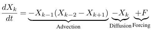
The first term on the right hand side is an advection term, while the second term represents damping. F represents an external forcing term, which is set to 10. Because this is a periodic system we can visualize it’s evolution in a circular plot:

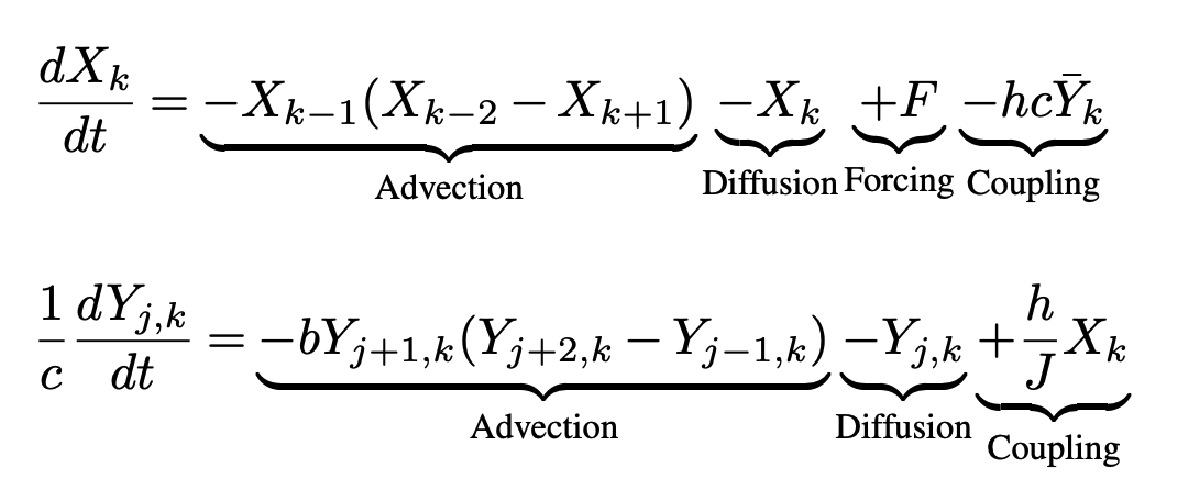
For parameter estimation or parameterization research, it is most common to use the two-level version of the L96 model. For this we add another periodic variable Y with its own set of ODEs. The X and Y ODEs are linked through coupling term which is the last term in both equations below. Each X has J Y variables associated with it.

Again, we can look at a visualization to better understand what’s happening.

Why the L96 model is too easy

Since its conception, the L96 model has been extensively used in data assimilation and parameterization research. Recently, the L96 models has experienced a resurgence to test drive machine learning algorithms for parameter learning or sub-grid parameterizations. In fact, I have recently published a paper myself, in which I demonstrated an online learning algorithm using the L96 model.

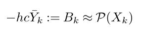
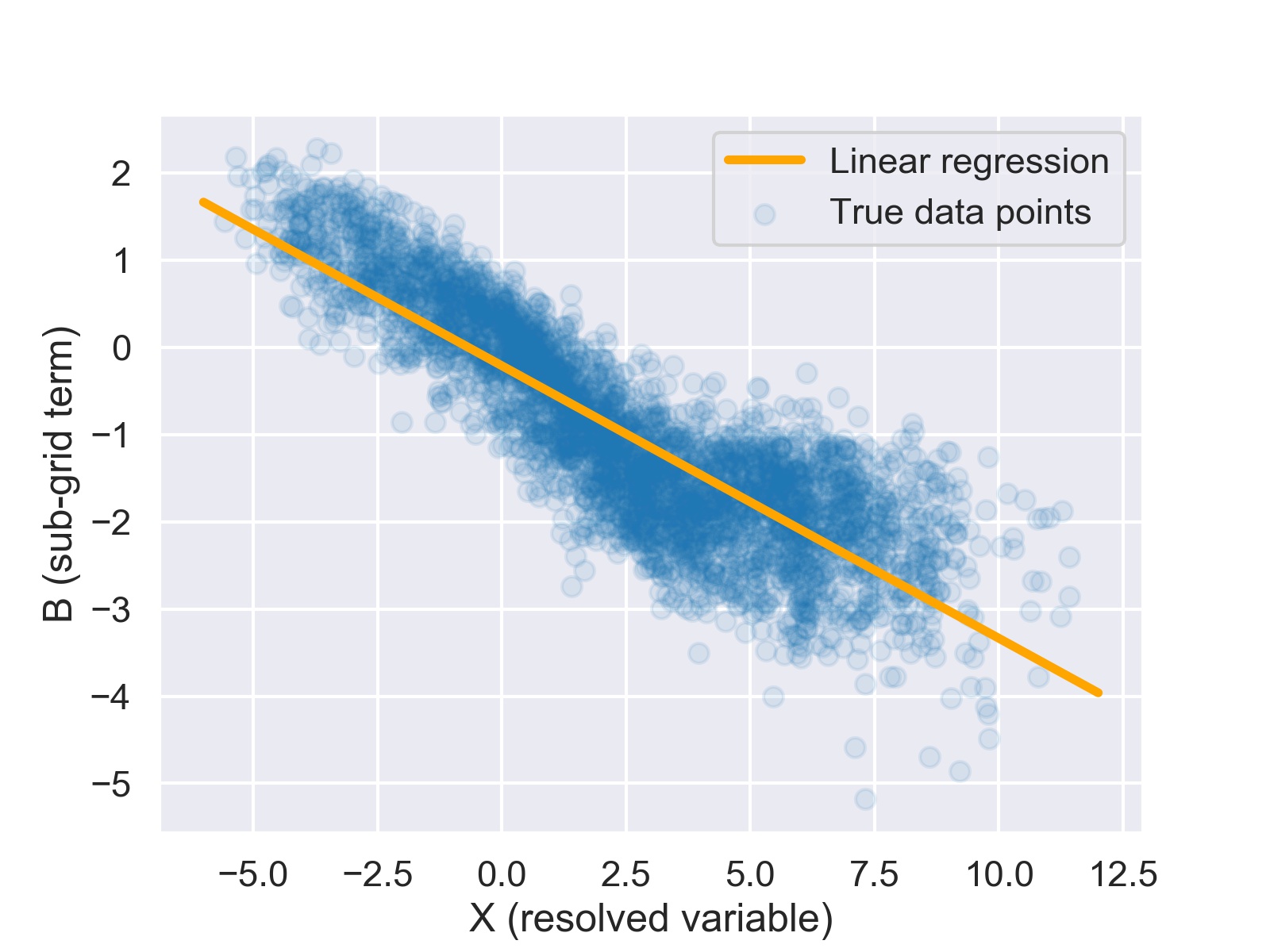
But there is one huge problem with L96: It’s too easy! What do I mean by that? Let’s look at a classic use case of the L96 model, parameterization research. In analogy to the real atmosphere or ocean, X represents the resolved, slow variables, while Y represents the unresolved, fast variables. Essentially, the task is to build a parameterization that represents the effect of the fast variables on X by replacing the last term in the X equation which we will call B for convenience.

Let’s assume that we are ignoring correlations in space and time and only modeling B_k as a local function of X_k.

The simplest parameterization, we can build is a linear regression:

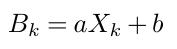
Here is what the true data points and the linear regression look like:

Now let’s use the simple linear regression parameterization, plug it into the L96 model and integrate for 100 non-dimensional time units. Here are the resulting statistics of X and B:

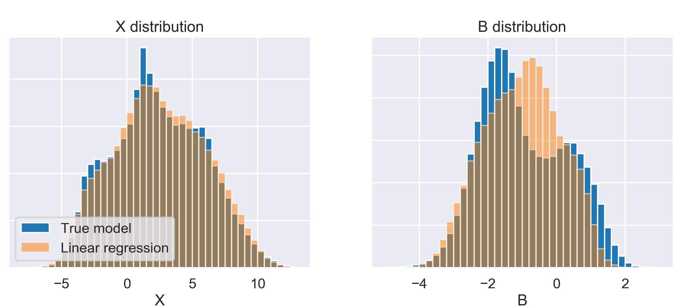
Of course, they are not identical but the differences in the X histogram are already very small. We can further compute some statistics like the mean and variability of X and B for the true and the parameterized models.

	Mean(X)	Var(X)	Mean(B)	Var(B)
True model	2.40	12.21	-0.95	1.57
Linear regression model	2.52	12.43	-1.00	1.22

The relative differences are really very small. This means that a simple linear regression basically solves the L96 parameterization problem. Of course, you can improve upon this simple baseline but we are experiencing none of the problems that plague ML parameterization research in real atmospheric or oceanic models.

The need for a more realistic toy model

Parameterizing sub-grid processes is the big challenge for climate modeling. Modern machine learning approaches could be one way to make real progress. Over the last two years, first studies (here and here and here) have demonstrated that it is generally feasible to build a ML parameterization. But, as I’ve summarized in my recent paper on online learning, there are several fundamental obstacles to overcome before ML parameterizations can actually improve weather and climate predictions. Stability, physical consistency and tuning are just some of them.

To tackle these issues we need to try out a range of new approaches. L96 can be a good starting point to make sure the algorithm works at all. But what if it does? Because L96 does not exhibit any of the problems that make more sophisticated approaches necessary in the first place a working implementation in L96 does not give much evidence whether the method will also work for full-complexity models.

So why not implement the algorithm in a full-complexity model right away then? The issue is that current atmosphere and ocean models come with huge technical baggage. They are typically written in hundreds of thousands of lines of MPI-enabled Fortran. This makes quick testing of a new method basically impossible. Even implementing a simple neural network trained in Python is currently a challenge. Fortran-Python interfacing is possible but not particularly user friendly and fast. More complex approaches like online learning, reinforcement learning or ensemble parameter estimation would require more complex changes to the model. Lastly, full-complexity models, particularly if a high-resolution simulation is needed, are computationally expensive which makes quick experimentation very difficult.

All of these challenges cry out for an intermediate step between L96 and full-complexity models.

Properties of an intermediate complexity model

So what should this intermediate complexity model look like? Here are some requirements:

1. Multi-scale: Since we are looking to build a sub-grid parameterization, we need a system which we can divide into resolved and unresolved processes. Ideally it is a continuous system, so we can simulate the additional challenge of coarse-graining.
2. One dominant direction of motion: In the atmosphere and ocean, vertical motions are very different from horizontal motions. This is the reason that parameterizations typically act on columns. Mirroring this would be helpful in a toy model.
3. Complex enough to exhibit real problems: The first two years of ML parameterization research have revealed the following key issues. A good toy model should simulate most of them.
   • Stability: Coupled/online simulations often turn out to be unstable.
   • Biases: Even if offline (uncoupled) validation suggests that the ML parameterization accurately reproduces the sub-grid effects, online runs often show biases or drifts.
   • Physical consistency: In the real Earth system it is crucial that energy and other properties are conserved. (A recent paper led by Tom Beucler showed how to do this during neural network training.) It should be possible to write down certain conservation properties.
   • Generalization to unseen climates: ML parameterizations have so far been unable to extrapolate much beyond their training range. This means that one should be able to change the basic state of the model through external forcing.
   • Stochasticity: Most ML parameterizations so far have been deterministic which means that some variability of the real, chaotic system is missing. The model should therefore also be chaotic.
4. Easy to understand: One issue with most available models, e.g. LES or CRMs is that they try to represent the atmosphere as well as possible, which leads to complicated numerical methods and physical equations. The intermediate-complexity model we are looking for does not need to be an accurate representation of the real world. Simplicity is much more important. This applies to the basic equations as well as the numerical methods.
5. Fast to run: Some proposed approaches require many model runs, often in an ensemble. The intermediate-complexity model should be fast enough to run a forecast in at most a few minutes.
6. Easy to use: This is absolutely key. The model has to have a Python interface to be compatible with the most used ML libraries. One should also be able to run the model interactively in a Jupyter notebook, i.e. execute one step at a time and look at the fields.

I am not an expert in fluid modeling, so I am calling out for help here. What would be a good set of equations that fulfils all (most) of these requirements? It could be a system very close to the real atmospheric/oceanic equations (i.e. Navier-Stokes) or something completely different that has similar characteristics.

I believe that fast testing of new approaches is absolutely key to progress in ML parameterization research. Currently we are (or at least I am) hampered by a gap between too simple models such as L96 and full-complexity models.

PS: My suggestion

Here is my very vague idea: a 2D cloud-resolving model with the simplest equations possible. As super-parameterization and other early convection research shows, two-dimensional CRMs capture much of the essence of real convection. And, of course, 2D models are much faster than 3D models.

The basis for this model could be the anelastic equations of motion. The microphysics scheme could be a simple saturation adjustment scheme with only one hydrometeor species (liquid) that rains out above a certain threshold. Turbulence could be modeled with a first-order local K-closure. The surface would have a constant temperature and interact with the air through a simple bulk scheme. Radiation would only be represented through a constant cooling in the free atmosphere.

With this model, it would be possible to run a radiative-convective-equilibrium setup. But to make it more interesting and involve some large scale dynamics, one could imagine a setup like this crude drawing shows.

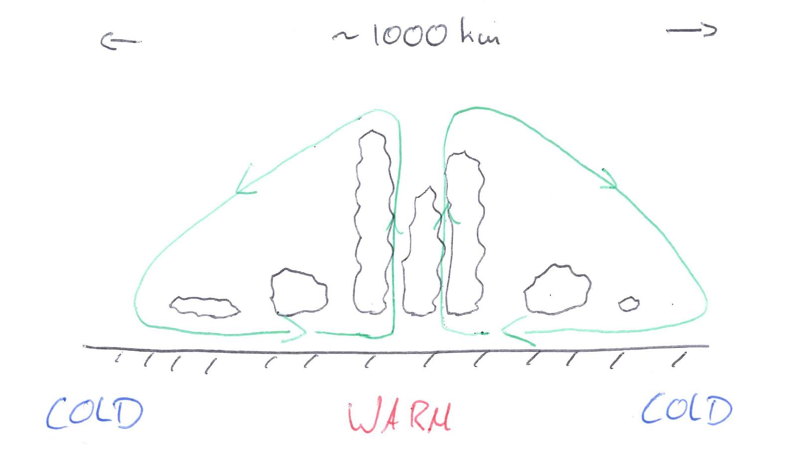
Here we basically have a flat, periodic mini-world with a cold-warm gradient that would induce a large-scale circulation cell with deep convection over the warm pool (right?). One could imagine a setup with 250 4km-wide columns with 30 levels. This should be manageable from a computational point of view.

Would this setup work and reproduce the key challenges outlined above? What should the exact equations be?